Predicting Lead Gen Revenue from a Book of Orders

Part 3 – Estimating Lead Gen Revenue

In the field of insurance, companies grow by building a collection of policies. This collection is called a Book. So an established and successful insurance agent will have a large Book of Policies. This Book defines the present value of the agent’s business. The agent will value his/her Book based on the current value of expected future commissions from policy renewals. Insurance carriers likewise build a Book of Policies and value the Book based on the estimate that collected premiums will be greater than claims on the policies, and that policies will probably renew, generating more cash and risk.

 

In the lead generation business companies build a Book of Orders for leads. This Book of Orders is an asset. The asset is depleted when the lead gen company obtains a lead from a consumer and sells the lead into the Book of Orders. The Book defines their capacity to generate revenue. This capacity is strictly determined by all orders in the company’s Book. So a rigid framework can be useful when describing the Book. Here X will denote orders and Y will denote Leads.

 

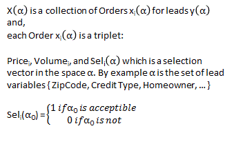Since the calculations are simple, we will adopt the full space of our selection variables in alpha. As described earlier posts, the selection space can have very large number of possibilities. In our case we have identified a space of 180 million possibilities. Given that storage space is cheap, it is advantageous to keep some Order information stored in this high resolution form. So this Selection functional is stored in full resolution for each order and for the Book.

So the value M that is the number of possible matches any given lead will produce. If M = 0 then there are no orders that match the lead. If M > 0 then leads will have matching orders.

 

Multiplicity M

When M > 1 for a given lead, the company can sell the same lead more than once. Multiplicity increase revenue and matching options for the company. So if a Book has, for a given lead, multiplicity of 3, revenue will depend on the matching policy. The policy may limit matches to 2 matches per lead. This is a common constraint in the lead gen business which is intended to control quality. Revenue depends on the lead matching policy.

 

In many cases lead matching is done to produce maximum revenue. The only constraint that a maximum of J matches are made. J=4 is a common policy constraint.

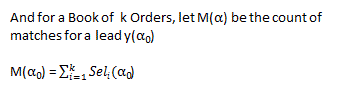
The revenue generated by a Book of Orders is well defined when all values of alpha are known and a conversion has occurred. But the information about the user is only known after conversion. Let’s go back to a Bayesian Network describing our process.

Imagine this fictitious Bayesian Network which was learned from our data. The top left cluster of nodes are our alpha nodes. The green nodes are Do variables. Each needs an optimal Do Policy so that Expected Profit will be maximum. Yellow nodes indicate hard evidence (values are known). So in our example, we know, ZipCode(Zip), and Currently Insured(CI) and Time of Day(TOD).

 

To simplify notation rho is a response variable. All seven response variables are relabeled.

 

Now what is the optimal Do Policy? Given what we know, we want to pick the bid (rho 1) for each ad (rho 2) and each Landing Page (rho3) so that Expected Profit from lead sales is greatest. Here we use a simple cost per click to model cost.

 

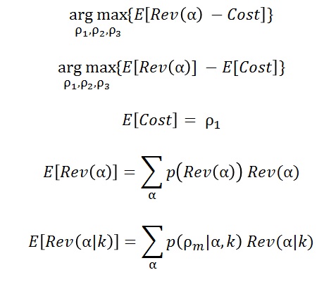The left hand side of the last equation above reads” The Expected Revenue given knowledge k.”  Expanding notation by being explicit:

 

Graph Mutilation (DAG Surgery)

Using Do calculus to eliminate variables by d separation and adding known values, the mutilated DAG for the Bayesian Network for rho becomes this. This vastly simplifies the probability distribution and the number of parameters required for the calculation.

 

It is important to remember the size of our original problem. It was immense with as many parameters as number of vehicles in the US.

 

This probability distribution is written directly from the mutilated DAG.

 

Now we have a prediction formula for conversion that only has 4 tables!! Only one appears to be large. Notice that rho 1 (Ad Bid) is not part of our distribution. Its effects on conversion are ‘cut off’ once we also intervene by doing rho 2 (intervening with an Ad).

 

 Expected Revenue

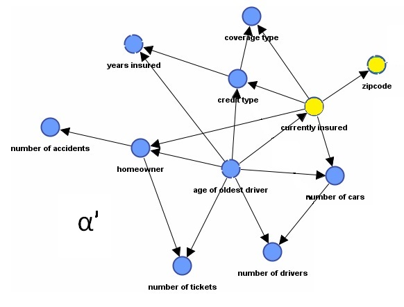Given we know Zip and CI, we will mutilate the DAG of our selection variables. This will produce a new distribution for the remaining variables in alpha. We will call the new distribution alpha prime.

 

Notice that once Currently Insured (CI) is known, ZipCode is cut off from the DAG. This vastly reduces the number of parameters needed to describe alpha prime. To speed operational calculations, two distributions can be pre-calculated: one for CI=T and one for CI=False

 

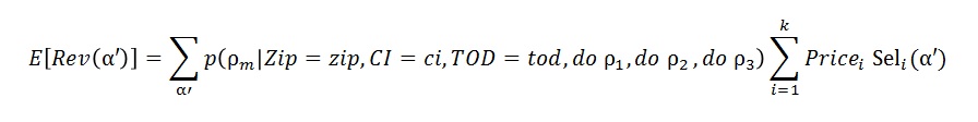
This updated distribution is used to estimate revenue from the Book of Orders. So that the calculation is:

 

This gives an explicit calculation for expected revenue given the Do variables. We are assuming that costs are based on a cost per click (per landing page view). So now we can calculate the optimal Do Policy using the following:

 

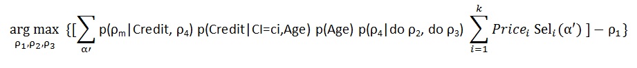
Notice that the last summation in the formula is our representation of the Book of Orders. It answers what orders we have in our subset space alpha prime. By keeping these records pre-calculated one can speed the optimization calculation.We can make optimal bids and choose the best Ad and best Landing page. The remaining question is can these calculations be done quickly enough? Less than 50 milliseconds would be a great user experience.

 

The revenue from clicks rho c1 and rho c2 have not been included in this solution. It would be a simple matter to model the Revenue from these outcomes and add them to the optimization formula.

 

If you see corrections or suggestions, please add a comment below.