For a long time now, I have been interested in modeling of businesses. In particular the SureHits business model of a click marketplace.
When we sold SureHits in 2008 to Quinstreet I worked with a banking analyst who built a giant spreadsheet that described the history of sales and projection of future sales. This spreadsheet/history held all of the microparameters of the business – sales to each customer, operating expenses and details of all our sources of clicks. Macroparameters like Sales last quarter and gross profit margins and EBITDA are very helpful measures of the business, but I wanted more. What macroparameters are important to SureHits success and value? Are there macroparameters about the history of sales and history of supply that can describe business risk and sustainability?
The resulting model using these microparameters made predictions based on many, many assumptions about customers, sources and expenses. I wanted a model that was more meaningful. I wanted predictions that were based on the ‘laws of accounting’ and ‘the laws of nature’ or some other fundamental principle. The goal of this thinking is to find a way to adjust the sales to each customer in a way that ‘stabilizes’ the system so that it will operate with minimum price volatility while producing good profit. If we model the system as an open thermodynamic system then we can use (MEP) the maximum entropy production principle to identify the best, most stable sales distribution.
Maximum Entropy Production Principle
The proposed principle of Maximum Entropy Production (MEP) states that the steady state of open thermodynamic systems with sufficient degrees of freedom are maintained in a state at which the production of entropy is maximized given the constraints of the system. A steady state system (at equilibrium) will have the most predictable performance. A stable system is prefered by customers, suppliers and investors.
This paper will show that maximum sales entropy production denotes this equilibrium point. If we can estimate future free cash flow + current free cash flow then this can be the new company goal: Produce the maximum equity each period.
 Business modeling and thermodynamics
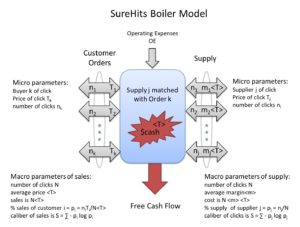
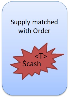
To build a model, apply the laws of accounting with the first law of thermodynamics to model the business as a reaction chamber. This picture of the boiler shows the inflows and outflows of the boiler.
The business generates free cash flow (free energy) by matching Orders for clicks from customers at price T
i from a Supply of clicks with cost (mT). The cash produced is = T – mT
i. For all possible matches in Customer Orders, when x is in x’, there exist potentials (1-m)T
i for each match. The Temperature of the boiler is <T> or expected price.
Current accounting reports
It is no surprise that the first law of thermodynamics is among the rules of accounting. Energy is neither created or destroyed. Cash is free Energy. The following financial reports are each bound by the first law and present a wealth of macroparameters for managers and investors.
Cash Flow (Sum of free energy)
Begin Cash + Cash from Operation – End Cash = 0
Income Statement (free energy production)
Sales – Cost of Goods Sold – Operating Expenses – Profit = 0
Balance Sheet (sum of all energy)
Cash + Goodwill – Liabilities – Equity = 0
Sales Entropy and Goodwill Statement
A new core financial report is suggested in green to show an accounting approach of the business model. The Sales Entropy and Goodwill Statement gives metrics that show what the
future may hold for the company. If Sales Entropy production is negative, then the company is depleting future sales for current sales and future price <T> will be more volatile. If Goodwill is depleted, then a charge against Goodwill is made. If Goodwill is produced then this value can be added to the Goodwill entry in the Balance Sheet and company Equity increases.
Now let’s set some initial conditions on the business model. Let liabilities and beginning cash be zero for the first reporting period. Let’s also plug in our equations for the diagram of the boiler model above.
Cash Flow (sum of free energy)
Free Cash Flow = End Cash
Income Statement (free energy production)
N<T> – m<T> – OE = Free Cash Flow
Sales Entropy and Goodwill Statement (
potential energy production)
End Sales Entropy – Begin Sales Entropy = Sales Entropy produced
S(t) – S(0) = Δ S(t) = Sales Entropy produced
<T> Δ S(t) =
Goodwill produced (potential energy)
Balance Sheet (sum of free energy and potential energy)
Free Cash Flow +
Goodwill = Equity
To measure this potential energy (that I’ll call Goodwill) we use the definition of Entropy, S, which states that the change in energy is the product of system temperature and the change of entropy. dU = TdS
Goodwill is potential energy. Goodwill is generally a expected sum of sales at some
future time from the customer base and reflects confidence in future sales. If a company buys another’s customer base, this asset is recorded as Goodwill. When a company produces it’s own sales base the stock market rewards them with higher company value (equity). To account for this value we should have one more core report for the business.
If Goodwill = Sales x Sales Entropy = N <T> S, then
Equity = FCF + N<T>S = N <T>(1-<m>) – OE + N<T>S
Equity = N <T> (1 – <m> + S) – OE
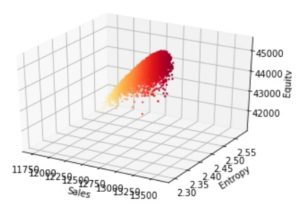
Equity will be maximum when d(Equity) / dT = 0 and when d(Equity)/dS = 0. To the right is a graph of this optimum using the price vector T from example below.
System Constraints
The marketplace has certain rules that place constraints on the system:
Constraint 1: If T1 > T2 > … > Tk then n1 > n2 > … nk
First clicks are auctioned based on bid price T so that a higher price will get more clicks than a lower price.
Constraint 2: dn/dT > 0 for all customers
If a customer increases bid price then the customer will get more clicks. Lowering bid will reduce clicks. Said another way: Price elasticity must be positive. (
This seems like a corollary to #1 above. If #1 is true, it follows #2 is true. Hmmm)
Constraint 3: Budget k ≥ nk <Tk>
Customers may have a maximum budget for the next time period. Sales produced cannot exceed Budget. Customers with budget constraints are not included in Constrain 1.
Two Example Sales Distributions
Let’s look at a few plausible sales distributions and calculate the Goodwill of each. The first is maximum sales and the second is an ad driven distribution. Which has highest Equity?
Maximum sales is result of giving all clicks to the highest bidder. If Tmax = $18.00 (as in examples below), the average <T> = $18 but no goodwill is produced since Sales Entropy = 0. The Equity = $18 + $0 = $18. Distributing all clicks to a single customer gives rise to the least stable system and price volatility is greatest.
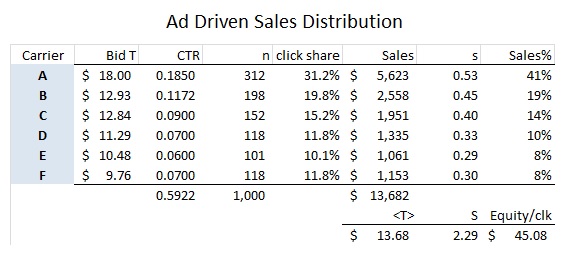
An ad driven sales distribution produces much more equity for the company by distributing clicks to every customer. The boiler operates at a lower <T> of $13.68 and it has sales entropy of 2.29 bits. The Goodwill of the sales distribution is $31.40 and has total equity of $45.08.
Clearly, the sales distribution is well connected to the total value of the company. So if the company has a set of bids
T, how do they best distribute clicks so that the sum of Free Cash Flow and Goodwill is greatest? As a starting point, our single market where the 6 customers bid for clicks. In this example the top bidder is much higher than all others and will get the greatest share of clicks.
MEP driven Optimization
 A simple Python algorithm
 is used to help find the sales distribution with highest equity. It applies noise to a beginning distribution by changing the number of clicks each customer receives.If the new distribution has higher equity and passes constraint 1, then that distribution is reserved and replaces the original distribution. The test is run many times.
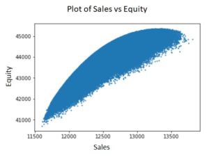
Here is an example of the results from running the algorithm once. A scatter plot of the random test reveals an optimum point of maximum Equity. The distribution with the greatest equity is saved (as best) and the experiment is repeated with less noise. With a few iterations of this process a nice peaked curve will be found. The peak is found where d (Equity) / d(Sales) = 0. The Equity peak also occurs when d(Equity)/dS = 0.
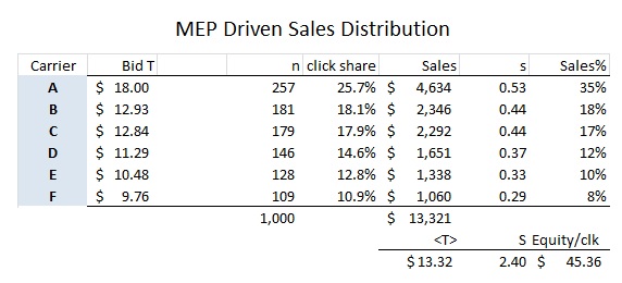
Using this algorithm the sales distribution that produces the maximum equity was found. In this example very modest changes were needed to the sales distribution. Again the average temperature is reduced to $13.32 (a 2-3% decline from ad driven).
The MEP solution reduces the share of sales to the highest two bidders which reduces future sales risk from these customers, especially carrier A whos market share drops 6%, A and induces more Goodwill and sales momentum from the lower ranks of bidders.
Conclusion
This paper has shows that sales to a customer base produces two types of Energy. FCF is free Energy and Goodwill is potential Energy. Investors and intelligent marketplace managers take a long view of value by including future sales and future price volatility into their decisions. To improve transparency investors and managers need a Sales Entropy and Goodwill Statement each period.
The Minimum Entropy Production Principle offers a way to find the ‘
best’ boiler operating Temperature <T> so that the value the boiler
will produce is at maximum. Burning too hot, giving all clicks to A, eliminates all sales momentum for all other carriers. If carriers B-F drop out of bidding, price will plummet since price elasticity for carrier A = 0 = dn/dT. At this point no market exists and Goodwill is zero.
MEP is said to offer a way to find the second and third order laws of how our boiler will behave. It would identify forces acting on the system and how these forces affect n of a supplier and T of a carrier. Is there an optimum margin m to give to suppliers? Can the collective ‘Supply’ be modeled to show the likely impact of price volatility ΔT on total clicks N.

 If Goodwill = Sales x Sales Entropy = N <T> S, then
Equity = FCF + N<T>S = N <T>(1-<m>) – OE + N<T>S
Equity = N <T> (1 – <m> + S) – OE
Equity will be maximum when d(Equity) / dT = 0 and when d(Equity)/dS = 0. To the right is a graph of this optimum using the price vector T from example below.
If Goodwill = Sales x Sales Entropy = N <T> S, then
Equity = FCF + N<T>S = N <T>(1-<m>) – OE + N<T>S
Equity = N <T> (1 – <m> + S) – OE
Equity will be maximum when d(Equity) / dT = 0 and when d(Equity)/dS = 0. To the right is a graph of this optimum using the price vector T from example below.
 A simple Python algorithm is used to help find the sales distribution with highest equity. It applies noise to a beginning distribution by changing the number of clicks each customer receives.If the new distribution has higher equity and passes constraint 1, then that distribution is reserved and replaces the original distribution. The test is run many times.
Here is an example of the results from running the algorithm once. A scatter plot of the random test reveals an optimum point of maximum Equity. The distribution with the greatest equity is saved (as best) and the experiment is repeated with less noise. With a few iterations of this process a nice peaked curve will be found. The peak is found where d (Equity) / d(Sales) = 0. The Equity peak also occurs when d(Equity)/dS = 0.
A simple Python algorithm is used to help find the sales distribution with highest equity. It applies noise to a beginning distribution by changing the number of clicks each customer receives.If the new distribution has higher equity and passes constraint 1, then that distribution is reserved and replaces the original distribution. The test is run many times.
Here is an example of the results from running the algorithm once. A scatter plot of the random test reveals an optimum point of maximum Equity. The distribution with the greatest equity is saved (as best) and the experiment is repeated with less noise. With a few iterations of this process a nice peaked curve will be found. The peak is found where d (Equity) / d(Sales) = 0. The Equity peak also occurs when d(Equity)/dS = 0.