Tag: hamiltonian

  • Business Energies and Potentials

    Business Energies and Potentials

    A business accounting and planning model will include 4 different types of business energy. I use the words ‘energy’ and ‘potential’ because they fit perfectly with business. This language also fits into current accounting practices with minor adjustment. Most importantly the language enables use of powerful prediction , planning and optimization mathematics for a business.

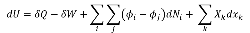
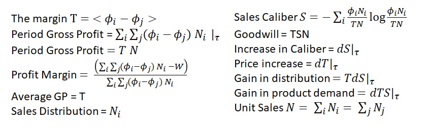
    Here are the four types of business potentials written in the form of the Fundamental Energy Equation for Business in terms of Potentials:

    Fundamental Equation of Business Potentials

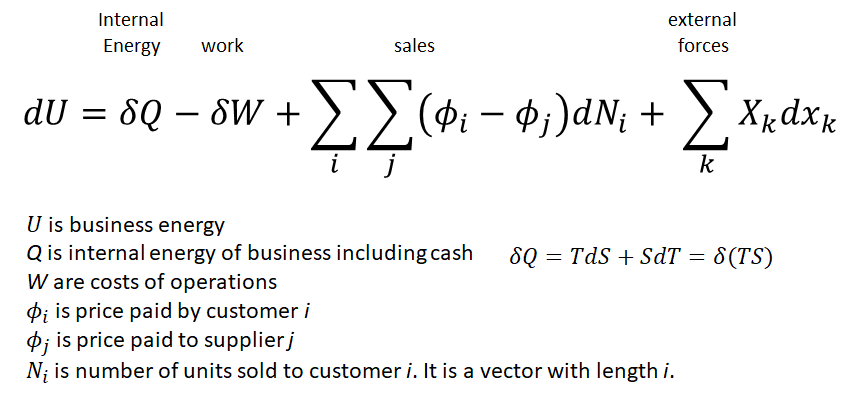
    The four business potentials are internal, work, sales, and external forces. In this blog each of these potentials are described with examples.

    Internal Potentials

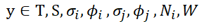
    The Natural variables of Business are Cash, T, S, W, Phi i, Phi j and N. Any force that causes change of a Natural variable is a potential. The sum over time of a potential ‘acting through some Natural distance dx’ is energy.

    Free Energy

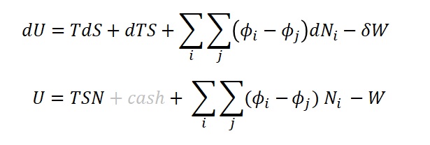
    Cash is the most simple of these. Cash is socialized free energy. Cash and accumulated free cash flow are free internal business energy. Cash energies are accounted for in GAAP as company current assets. All other internal energies are potential energies.

    Example: Any bank account with instant no cost access to cash for the Business is Free Energy.

    Potential Energy

    Typically other Inventory, Equipment, and Plant assets are another form of potential energy which can be potentially sold for cash. These energies are recorded as Tangible assets in the company books and depleted through amortization and sales.

    Example: A Unit of product in inventory is a Potential Sale and its Cost as its Potential Energy.

    Example: A desktop computer is purchased for $1,000 cash. Each year the energy is used up through employee use. At end of year 1, $200 is lost as Work and $800 remains as Potential Energy.

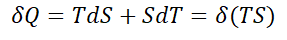
    There are two other types of potential energies: TdS and dTS. Over a time period, these potentials combine to form the potential energy TSN.

    Example: The “Book of Sales”, describing customer sales over a time period is internal potential energy. The internal energy of the Book of Sales = TSN. It is predicted future sales.

    The first of these types, TdS, are the changes to sales caliber S, where T is expected profit margin. These quantities of change are seen in Intangible assets or in Shareholder Equity. These assets help the company increase distribution. If the asset is acquired through M&A it is reported as Goodwill. All others are recorded as Shareholder Equity. This makes TdS an important energy to Investors!

    Example: Business acquires 10 new customers and sells each optimum product quantities. This increases Shareholder Equity by a factor dT dS.

    Example: Business acquires 10 new customers by purchasing a company and sold each optimum product quantities. This new business may change T, S and N for the business. Sales, Goodwill and Shareholder Value are affected.

    The term dTS are the Intangible assets/potentials in the company that increase margin T with fixed Caliber S. These are assets that give the business a price advantage in the market. It could be low cost mineral in a company owned quarry. It might be a lease that gives ability for the business to produce cheap products. It might be greater access to N such as media share.

    Example: A Patent that gives a business production, processing, or pricing advantage.

    Example: Key Person Potential. Professional employees are often considered assets of business practices such as programmers, Lawyers, Medical Doctors.

    Company Work Potentials

    Expenses needed to run a business are the result of Work potentials. They drain cash out of the company. They also support company employee wages and benefits. These expenses (energies) help company departments achieve their goals.

    Example: A company buys product in bulk and Works to repackage the product into smaller units in order to get a higher T and higher Sales. This is a Work Potential on dT and d(Sales).

    General and Administrative supply company admin and security. It seems that all other work is directly related to improving T, S and N. Sales and marketing work to improve T, N and S. Engineering and development efforts may also work to improve market advantages on T, S or N. Engineering and Sales also spend money/energy to improve conductivity rho of business between customers and suppliers alike.

    Sales Potentials

    The ability of the business to operate with a positive margin are the sales potentials that it develops, customer i paying phi i per unit dN. Each customer represents a potential and each customer will produce different levels of potential.

    Example: Customer 5 will pay $60 for a unit that costs $50. This is Sales Potential of $10.

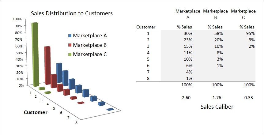
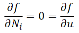
    If the sales potentials are ordered by magnitude, greatest to least, and we take the gradient of these potentials we find a great tool for managing the optimal distribution problem, which is: How do I choose which customer gets unit n when prices vary from customer to customer? The business wants to make the most profit AND wants to have a large, diverse customer base. They want maximum Sales plus Maximum customer goodwill. They want max (Sales + Goodwill) which is max(TN+ TSN)

    It turns out that the gradient of the sales potential is a key to solving this problem. If all prices are the same, gradient of sales potential is zero, then optimally the sales distribution is flat and each customer gets same volume N, produce same margin T, and same Sales TN.

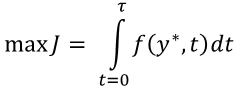
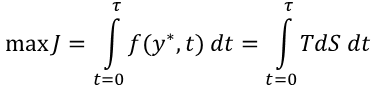
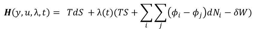
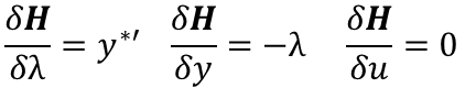
    But in many businesses the gradient of the sales potential is not flat and managers must solve the distribution vs profit dilemma. The Business Hamiltonian of the Business performance goal and the Business Energy Equation offers a solution to the dilemma. It offers a simple set of calculations that determines the optimal sales distribution given any sales potential gradient.

    External Forces

    For an external force to impact the energy of the business, the force X must ‘act through some distance’ dx, where x is among {T,S,N,phi}. The force must act on the one of the first three terms (Internal Energy, Work, or Sales) of the energy equation to affect the company’s performance.

    Example: Business tax rates are a negative external force on Sales which becomes a Work potential. A tax rate lower than the competition may be seen as a positive ‘relative’ potential giving the business an advantage.

    The ambient temperature phi of a product market is a force that will affect all businesses except monopolies. Each customer will have other options to conduct business to purchase N units. The ambient Temperature of the market will place a force on the prices customers will pay, pushing low prices up and high prices down toward a average/ambient price.

    Conclusion

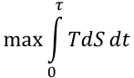
    By making this simple assumption “Cash is socialized free energy”, business can be described as a machine whose future states are predictable and controllable. The machine is designed to produce free energy for investors. A very good goal for any business would be to produce the greatest total energy over some time period. Here I hoped to show that accounting for intangible energy asset TSN is vital for investors and managers alike who care more about consistent sales in future periods than the current period sales.

    After establishing a performance goal of the company a Hamiltonian can be written and solved showing the predicted future states of the business.

    References

  • Fundamental Equation of Business Potentials

    Fundamental Equation of Business Potentials

    Since I was a student of mechanics and physics a better understanding has emerged. Hamiltonian and Lagrangian math has revealed a single method from which the “Laws of Nature’ can be derived. The method is to choose a coordinate system, write the Hamiltonian, assume some initial conditions and then solve the “Saddle” equations. This calculus has been used to derive Newton’s Laws of Motion. It solves 3 body celestial problems, solves any mechanical device’s future motion, it explains solutions in quantum mechanics, all of Maxwell’s equations, Kirchhoff’s principles, Fourier’s heat transfer. I have not seen this math applied to business.

    The Laws of Motion of business would predict future states of the business. This math could be very helpful to managers wishing to obtain better performance from the company. Since business is the practice of goal seeking they really want to control the business so that some performance is maximum. Hamiltonian math can find the optimal control u(x,t) that will produce maximum performance. It also can produce the trajectory of variables in business. These are the laws of motion.

    To begin we need to pick a coordinate system that will describe the business. Business already uses a host of metrics to account for its states. The English language surrounding business also seems a natural fit for the problem. The main coordinate for business is cash. Let cash be free Energy. Free cash flow is a company’s production of Free Energy.

    Energy, Entropy and Temperature

    The physical world is well described using models that involve Temperature, Entropy and physical coordinates (Voltage, pressure, volume, conductance). A Carnot Heat Engine is a simple model of how to extract Work from a Temperature potential. Here entropic forces generate work from a machine between two temperatures. Electric circuits dissipate energy when entropic forces push current through an conductance. Potential energy causes current to flow through the conductance which dissipates energy. This figure models a business using the same language (coordinates).

    Imagine businesses are bubbles that conduct business by touching after agreement on terms: N, t, and price. This price is phi. Rho is the conductance that allows a given flow rate. The product of N and phi is cash flow or change in energy. Likewise I think a model business will include Entropy along with business metrics (Sales, Costs, Budget, Market Cap, Goodwill, Risk) and can be very helpful for making decisions.

    Fundamental Equation of Business Potentials

    For a time period τ the change in value of a business dU is the change in internal energy less the cost of work plus the change in sales plus changes forced by external variables.

    U is business value
    Q is internal energy of business including cash
    W are costs of operations
    ϕ_i  is price paid by customer i
    ϕ_j  is price paid to supplier j
    N_i, is number of units sold to each customer i. It is a vector with length i.

    Sales Sustainability and Sales Caliber

    Investors and business managers insist on sustainability. They hate risks to ongoing sales. Business managers reduce sales risk by selling to many customers and then distributing sales to its customers. I propose using Sales Caliber as a measure of a business’s sales sustainability. Sales Caliber is the Shannon Entropy of the Sales Distribution (named “Caliber” by E.T. Jaynes).

    Three example sales distributions are shown below. Business/Marketplace C has fewest customers and 95% of sales are to one customer (intense sales concentration risk):

    Caliber of Sales, S, is a direct measure of the certainty of future sales. Likewise, 1/S, is the Risk of future Sales. If T is profit margin, then TSN represents business’s potential energy from future sales. Caliber is a continuous measure of sustainability making it a very helpful metric for business managers. Said another way:  Goodwill = T x Sales Caliber x N

    The change in internal energy is the sum of the margin T times change in Caliber S plus the Caliber S times the change in margin T.

    Business Value as Total Energy

    If we take the Fundamental Equation, substitute the above, and integrate over time tau or over N, we get:

    These equations simply sum the energy provided the business in the form of potentials. These are the energy equations of business with external forces excluded.

    Business Performance Measures

    Most of standard business metrics can be found by knowing the value of each variable in the energy equations. Here is a selection of business performance metrics.

    Optimizing Business Performance

    Every business is seeking a goal and I think success comes mostly to business with well considered goals. Here are the variables of the business:

    Not all of these variables are accessible to the business. Example, in an auction setting the customer sets the price phi i. Typically some performance J is to be maximized over the next month, quarter, or next several years (over some time period τ).

    Imagine that the goal of a young business is to produce maximum TdS each quarter whatever other y may become. Then the performance function is:

    f(y,t)=TdS. The business does this by changing the vectors σi and Ni  . This maximum can be computed very quickly and will have an optimal Ni  * distribution of product given the goal.

    This maximum occurs when the partial derivative of f with respect to Ni is 0. Ni is our control u below:

    This solution was very easy with no constraints. Real business goals most often have constraints of allowable business states. In the above J we might add a constraint that gross profit margin T must be > 13%. But still the last expression is true del f /del u = 0

    Another goal might be to maximize gross profit. To accomplish this goal, the entropy of the business is depleted (exemplifying that it is potential). To maximize gross Profit by adjusting Ni, we simply deliver all N units to customer with greatest price ϕi. The entropy of such a distribution is 0, produces maximum temperature T and is least sustainable state of the business with S=0. This is a bad goal without constraints.

    The Hamiltonian

    Now that we have a general form for performance J and the energy equations of business, we can write the Hamiltonian:

    with performance function f:

    The Hamiltonian is:

    If a pair (u*(t), y*(t)) is optimal then there exists a continuously differentiable function λ(t) such that:

    Business Laws of Motion

    These partial differential equations predict the final state of the business when management applies changes to a control. In our example the control u is Ni, and the prediction is the optimum Temperature and change of Entropy (T*,dS*) given the performance goal of the business. They are a way to calculate values of all other variables of the business model at time:

    The function λ(t) is a Lagrangian transformation. We begin finding the optimal control using the last equation and then calculate each other variable in y using the first two equations.

    To be clear, a business has a limited number of variables y that it can control and which describe it’s periodic performance. Any ‘law of motion’ will include the variables in the energy equation of the business. The laws of motion y(t) and y’(t) can be calculated by solving the Hamiltonian differential equations on a computer with Python. Those variables in y not in the control can be forecast or predicted.

    Lastly

    The equations of motion of a business predict the state of business after a time τ. By applying a performance function and the energy function (aka business potentials) of the business to form the Hamiltonian, we can then estimate the state of all other variables in the collection y.

    TSN + cash is the potential energy of a business. Free cash flow is kinetic energy.

    It is clear that a company should optimize it’s distribution of products to produce Entropy. “The goal of business is to produce entropy”. Who said that? Seems that in business Entropy can decline if managers choose to begin selling product to fewer customers or if customers choose to stop buying.

    A more modern accounting of business would include formal reporting of TdS and dTS, and TSN. Investors are more interested in future potential of the business. This is best estimated with the internal energy TSN which is the business asset Goodwill which encompasses: (price, distribution, volume).

    References

    1. Wayne, James J., 2013. “Fundamental Equation of Economics,” MPRA Paper 50695, University Library of Munich, Germany.
    2. Kirk, Donald,J., 1967, “Optimal Control Theory”, Prentice Hall
    3. Hamill, Patrick, 2014, “Lagrangians and Hamiltonians: A Student Guide to”, Cambridge University Press
    4. Jaynes, E.T., “The Minimum Entropy Production Principle“,
    5. WikiPedia, “Thermodynamic Potential“,