Ad Serving using Causal Inference

It has been a decade since we used very simple models for ad serving. Even then, with simple models, we produced great results. I did not realize it then, but we were using simple Causal Inference to make our estimates.

Causal Inference is a prediction

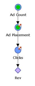
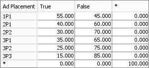
Our model was simple (Figure 1). When we could place several ads in a list, we just knew higher ranked ads got more clicks. Just as it happens in search engines. So Ad Placement completely determines the number of clicks and revenue. The Click node has a probability table that contains p(Click | Placement) – the probability of a Click given a particular Placement. The Table looks like this:

 

As we collected data on particular ads we could accurately predict probability of Click for any Placement {1st of 3 (3P1)=35%, last of 3 (3P3)=15%, second of two(2P2)=30%, etc}. The table can be updated easily with new data which is kept in the form of occurrences. The prediction this table provides is called Causal Inference.

 

Our customers would bid on placement in our system. It was our simple goal to produce the most revenue from every user. The model was used to predict revenue and another process was used to determine the final list of ads to be displayed.

 

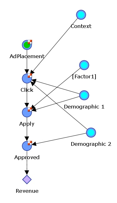
Modern ad servers have more complicated predictions. Some advertisers (Figure 2) want to reduce their risk by paying only when an ad produces an Approved customer. Now the consumer must complete an application and be approved before revenue occurs.

Expected Ad Revenue = Bid p(Approved|Apply) p(Apply|Click) p(Click|Ad Placement) p(Ad Placement)

 

Improving the accuracy of the prediction is important and will improve performance of the Ad Server. Figure 3 shows a Causal model that uses customer demographics and Context to improve the prediction. By using demographic variables, the Ad Server can customize the ads for a particular type of user. This can greatly increase performance.

 

When the server needs to add evidence (demographics and context) the calculation becomes a bit more complicated. Modern software can make these calculations very fast. Fast enough for Ad Servers. Simple algebra can be used to make the calculation too and is a matter of eliminating all unknown variables (Click and Apply) leaving an expression for the probability of Approved given Ad Placement, Demographics and Context. Either way, once the relationships are known and data is put in tables, fast accurate predictions of revenue can be made.

 

Each ad can be modeled. For the ad shown in Figure 3 there are 4 variables. Other ads with different consumer response will be different.

 

Modern software is used to learn the most accurate and least complicated models. A data set with past ad placements and responses, customer demographics and context is used for model learning. Ads for which little is known may have very few demographics in the model. When there is no data about an ad (a new ad) a general model can be used.

 

An Ad Serving Policy

 

Ad Serving is the decision process that selects from a collection of Ads and determines which set of Ads is expected to produce the most revenue. There are several types of decisions made:

1. Do I include this ad or exclude it from the set? Possible decisions: {Yes, No}.
2. For included ads, what is the Placement for each? Possible decisions: {nP1, nP2,  … nPn} where n is the count of included ads.

 

An ad serving Policy is a set of rules that will determine the answers to these decisions. The Policy includes the algorithm and tests used to make the decisions. One Policy might enforce that the maximum number of ads is 6 and no less than 2. Another Policy might search for the best ad for nP1 (first slot), make that decision and then look for the ad that will produce the most revenue in second slot (nP2) and so on until last ad is placed.

 

How do we find the “Best” Policy? The Policy most likely to produce the maximum revenue?

 

Intelligent Ad Serving

Even as simple as our model was 10 years ago, there were difficult challenges. Even if a maximum of 5 ads were shown, if we had 10 possible ads to display the possible combinations of Ad Sets was very, very large (100,000+ permutations). It is not feasible to calculate revenue for each possible combination of ads. We applied some ‘brute force’ assumptions and finally produced the best ad set (from a list of good choices).

 

A more modern approach employs the science of Entropy to make the decisions needed to produce the best Ad Set.

 

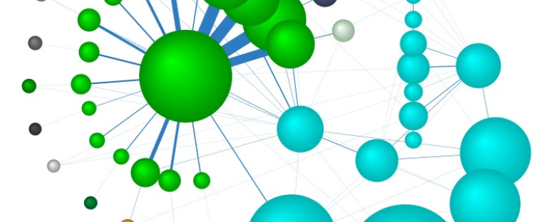
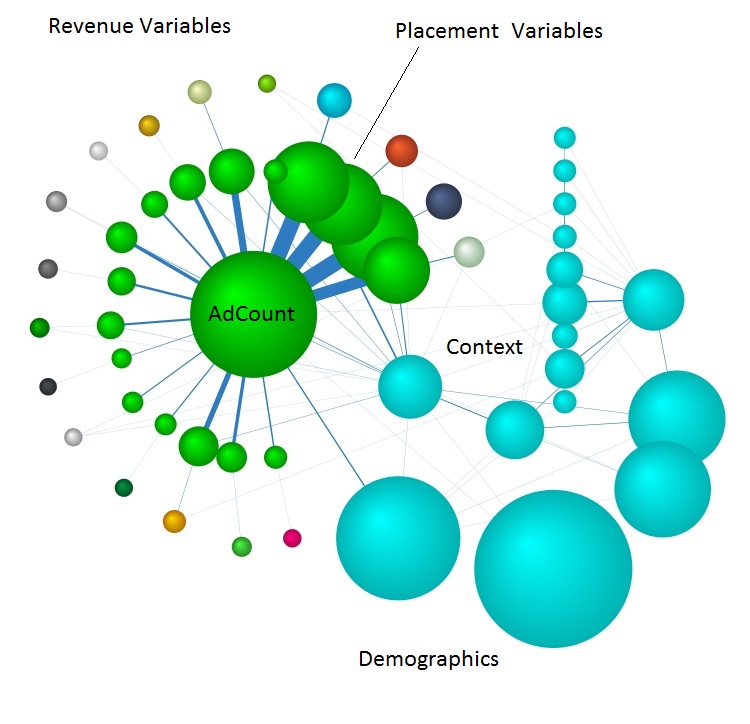
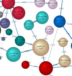
Figure 5 depicts the Entropy of variables (nodes) in a Causal model of an Ad Server. The size of each node is the amount of Entropy in the variable. In this graph the revenue variables surround the Placement and AdCount variables. The light blue variables are consumer demographics and context. This is the model when nothing is known about the user and no placement decisions have been made.

 

Once the Context and Demographic variables are set (known), the entropy of the nodes will shrink. Demographic and Context Entropy go to zero and other nodes Entropy is reduced. This gives us the starting system Entropy to begin making Ad Server decisions.

 

For a given Revenue node, the Entropic Force on revenue is the product of the Ad’s Bid and the node Entropy.

Force(Approved) = Bid ( – p(Approved) log p(Approved) )

The sum of these forces over all revenue nodes is Total Entropic Force on revenue. Intelligent strategies make decisions which maximize the change in Revenue per Change in Entropic force on Revenue. Here is an algorithm for making all decisions needed for Ad Serving.

1. Test inclusion or exclusion for each ad. Make decision that has most Change of Revenue per Change in Entropic Force. After setting the decision in the ad chosen for inclusion, repeat exercise on remaining nodes. Repeat until all nodes have a decision set. AdCount is decided and is limited to no more than K ads. Total number of tests at most are: 2N + 2(N-1) + … where N is the number of eligible ads to display.
2. Of the included ads, test to find the placement decision with greatest Revenue change per Change in Entropic force which meets the maximum ad count policy. Maximum number of steps = S x S  0r S^2 where S is the number of Ads selected for inclusion. Where S ≤ K where K is the maximum number of ads shown.

 

Conclusion

Causal Inference is making predictions using a Causal Bayesian Network as a model. These models can be learned from operational data and do not require experimentation to derive. Ads with no data history can be modeled using general models based on overall performance of ads or by expert opinion. Ad performance can be easily modeled with very few factors. Or for more accuracy Demographics and Context can be included in the model.

 

Intelligent algorithms based on Entropic Forces are very fast and quickly identify top performing Ad Sets. Since all of these causal inferences (calculations) needed for Ad Serving are available for free (as in R) or with technical support (like BayesiaLab Inference API and BayesiaLab Pro to learn models). Experts can also use experience to define models – just like our first model based on our expert confidence. Data can then be imported into the tables to provide inference.

 

These models are easy to implement and simple to update. More Ad Servers should use Causal Inference.

 

The images below are for another project in Kaggle.